Working with CSV or TXT datasets larger than RAM in R using SQLite


The RAM problem and enormous datasets
I do not know whether this happens to everyone, but whenever I start a new job, I seem to get the worst computer in the office: usually no more than 4 GB of RAM, and even 32-bit Windows if I am unlucky, as happened once. Since I use R for everything, large datasets can be difficult to handle, especially when they exceed the memory available to R. This tutorial also helps with enormous datasets.
We will check how much RAM is available to R and create a SQLite database. We can then retrieve manageable subsets and analyse them in memory, using a function I adapted from this gist by vnijs.
We will use SQLite because it is easy to configure and run locally. PostgreSQL and MySQL are alternatives, but setting them up would be a little more involved.
This tutorial assumes intermediate-to-advanced R skills and some familiarity with SQL.
First things first: how much memory is available?
To check the memory available to R, we will use the memory limit command shown below.
memory.limit()## [1] 16269I have approximately 16 GB of memory available, or about 16,000 MB—the RAM installed in this computer.
Note: On a 32-bit operating system, the memory limit cannot exceed roughly 2–3 GB, regardless of how much RAM is installed.
CSV or TXT to SQLite
Suppose we have a HUGE CSV or TXT dataset. I will use Chile’s 2017 Population and Housing Census. It is not exceptionally large, but works well for this example. You can download it from Chile’s National Statistics Institute.
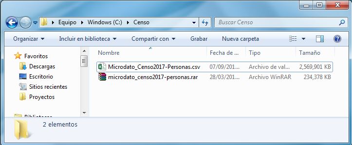
Extract the RAR archive to obtain the CSV file. It is approximately 2.5 GB—not enormous, but potentially too large for R on a low-spec computer. Opening it in Excel can also be difficult.
I will extract the dataset into a folder called “Censo” on the C:/ drive.
The packages you need
Make sure these five packages are installed:
- readr: to read comma-, tab- or otherwise-delimited files.
- DBI and RSQLite: to communicate with databases and use SQLite.
- dplyr and dbplyr: to retrieve information from the database.
library(readr)
library(DBI)
library(RSQLite)
library(dplyr)
library(dbplyr)
How large is the dataset, and what does it look like?
First, define the dataset path and assign it to delim_file:
delim_file <- "C:/Censo/Microdato_Censo2017-Personas.csv"To inspect the file, read its first two lines using readLines.
readLines(delim_file, n=2)## [1] "REGION;PROVINCIA;COMUNA;DC;AREA;ZC_LOC;ID_ZONA_LOC;NVIV;NHOGAR;PERSONAN;P07;P08;P09;P10;P10COMUNA;P10PAIS;P11;P11COMUNA;P11PAIS;P12;P12COMUNA;P12PAIS;P12A_LLEGADA;P12A_TRAMO;P13;P14;P15;P15A;P16;P16A;P16A_OTRO;P17;P18;P19;P20;P21M;P21A;P10PAIS_GRUPO;P11PAIS_GRUPO;P12PAIS_GRUPO;ESCOLARIDAD;P16A_GRUPO;REGION_15R;PROVINCIA_15R;COMUNA_15R;P10COMUNA_15R;P11COMUNA_15R;P12COMUNA_15R"
## [2] "15;152;15202;1;2;6;13225;1;1;1;1;1;73;1;98;998;3;15101;998;1;98;998;9998;98;2;4;6;2;1;2;98;7;98;98;98;98;9998;998;998;998;4;2;15;152;15202;98;15101;98"We can now see the column names and identify the delimiter: a semicolon (;).
R cannot count rows by loading a file that does not fit in memory. Instead, we will use a PowerShell command (Get-Content) on Windows, or a system command (wc) on Linux.
To count the rows in the file—this takes a little while:
On Windows:
total_records <- system2("powershell", args = c("Get-content", delim_file, "|", "Measure-Object", "–Line"),
                         stdout = TRUE)
total_records <- as.numeric(gsub("[^0-9]", "", paste(total_records, collapse = ""))) - 1
total_records
## [1] 17574003There are 17,574,003 records, excluding the header. That matches the number of people recorded by the 2017 census.
Note: Windows 10 should work without problems. On Windows 7 or 8, check your PowerShell version using these Microsoft instructions, and install PowerShell 5.1 by following this Microsoft guide.
On Linux, it would look like this:
 total_records <- system2("wc", args = c("-l", delim_file), stdout = TRUE) %>%
 sub(normalizePath(delim_file), "", .) %>%
 as.integer() %>%
       {
         . - 1
       }
Create the database path
Choose a path for the future database file, with the extension .sqlite3.
Define the database path and the table name. We will need the table name to retrieve data later. Another advantage of SQLite databases is that they can contain several tables.
table_name_censo <- "censo2017"
sqlite_file_censo <- "C:/Censo/censo2017.sqlite3"
The promised function
With the total row count, file paths and delimiter (comma, semicolon, space, and so on) identified, we can use the following function:
read_delim2sqlite <- function(delim_file, delim, sqlite_file, table_name, batch_size = 10000, OS = "Windows") {
establish a connection to the database
condb <- dbConnect(SQLite(), sqlite_file)
get the total number of records in the file
in Unix
if (OS == "Unix") {
total_records <- system2("wc", args = c("-l", delim_file), stdout = TRUE) %>%
sub(normalizePath(delim_file), "", .) %>%
as.integer() %>%
{
. - 1
}
} else {
# In windows
total_records <- system2("powershell", args = c("Get-content", delim_file, "|", "Measure-Object", "–Line"), stdout = TRUE)
total_records <- as.numeric(gsub("[^0-9]", "", paste(total_records, collapse = ""))) - 1
}
message("Total records: ", total_records)
find the number of passes needed based on size of each batch
passes <- total_records %/% batch_size
remaining <- total_records %% batch_size
message("Total Passes to complete: ", passes)
first pass determines header and column types
dat <- read_delim(delim_file, delim, n_max = batch_size, progress = FALSE) %>% as.data.frame()
if (nrow(problems(dat)) > 0) print(problems(dat))
col_names <- colnames(dat)
col_types <- c(character = "c", numeric = "d", integer = "i", logical = "l", Date = "c") %>%
.[sapply(dat, class)] %>%
paste0(collapse = "")
write to database table
dbWriteTable(condb, table_name, dat, overwrite = TRUE)
multiple passes
for (p in 2:passes) {
message("Pass number: ", p, ", Progress:", round(p / passes, 2) * 100, "%")
read_delim(delim_file, delim,
col_names = col_names, col_types = col_types,
skip = (p - 1) * batch_size + 1, n_max = batch_size, progress = FALSE
) %>%
as.data.frame() %>%
dbWriteTable(condb, table_name, ., append = TRUE)
}
if (remaining) {
read_delim(delim_file, delim,
col_names = col_names, col_types = col_types,
skip = p * batch_size + 1, n_max = remaining, progress = FALSE
) %>%
as.data.frame() %>%
dbWriteTable(condb, table_name, ., append = TRUE)
}
close the database connection
dbDisconnect(condb)
}
The function may look intimidating, but it is fairly straightforward. It reads the file in chunks of batch_size rows using read_delim from readr, inserts each chunk into the SQLite database, and repeats the process through the final line.
The function arguments are:
delim_file: path to the delimited file, in this case the census dataset. delim: delimiter character, a semicolon here. sqlite_file: path to the SQLite database, ending in “.sqlite3”. table_name: name of the table within the SQLite database. batch_size: number of records to read in each iteration. OS: the operating system, either “Windows” or “Unix”; the Unix option was tested on Linux, not macOS.
Move the CSV or TXT file into SQLite
We are ready to use the function. To avoid running out of RAM, I will transfer the dataset in batches of one million rows. It should finish in 18 iterations.
This will take a few minutes—time to make some mate!
read_delim2sqlite(delim_file, delim=";", sqlite_file = sqlite_file_censo,
                  table_name = table_name_censo, batch_size=1000000)
## Total records: 17574003## Total Passes to complete: 17## Parsed with column specification:
## cols(
## .default = col_integer(),
## P18 = col_character()
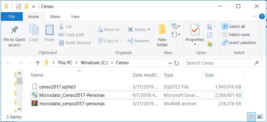
## )## See spec(...) for full column specifications.## Pass number: 2, Progress:12%## Pass number: 3, Progress:18%## Pass number: 4, Progress:24%## Pass number: 5, Progress:29%## Pass number: 6, Progress:35%## Pass number: 7, Progress:41%## Pass number: 8, Progress:47%## Pass number: 9, Progress:53%## Pass number: 10, Progress:59%## Pass number: 11, Progress:65%## Pass number: 12, Progress:71%## Pass number: 13, Progress:76%## Pass number: 14, Progress:82%## Pass number: 15, Progress:88%## Pass number: 16, Progress:94%## Pass number: 17, Progress:100%We only need to run this lengthy conversion once. It creates a .sqlite3 file that is slightly smaller than the CSV.
SQLite file created
Analyse and retrieve data with dplyr
To start retrieving data from the table, first connect to the database.
con <- dbConnect(SQLite(), sqlite_file_censo)
con
## <SQLiteConnection>
## Path: C:\Censo\censo2017.sqlite3
## Extensions: TRUEWe can inspect the connection details and the table name assigned to the dataset.
dbListTables(con)## [1] "censo2017"Create an object representing the data. It does not load the dataset into RAM: it is only a connection, which is why the total row count is not shown.
datos_db <- tbl(con, "censo2017")
datos_db
## # Source: table<censo2017> [?? x 48]
## # Database: sqlite 3.22.0 [C:\Censo\censo2017.sqlite3]
## REGION PROVINCIA COMUNA DC AREA ZC_LOC ID_ZONA_LOC NVIV NHOGAR
## <int> <int> <int> <int> <int> <int> <int> <int> <int>
## 1 15 152 15202 1 2 6 13225 1 1
## 2 15 152 15202 1 2 6 13225 3 1
## 3 15 152 15202 1 2 6 13225 3 1
## 4 15 152 15202 1 2 6 13225 3 1
## 5 15 152 15202 1 2 6 13225 3 1
## 6 15 152 15202 1 2 6 13225 9 1
## 7 15 152 15202 1 2 6 13225 9 1
## 8 15 152 15202 1 2 6 13225 9 1
## 9 15 152 15202 1 2 6 13225 9 1
## 10 15 152 15202 1 2 6 13225 10 1
## # ... with more rows, and 39 more variables: PERSONAN <int>, P07 <int>,
## # P08 <int>, P09 <int>, P10 <int>, P10COMUNA <int>, P10PAIS <int>,
## # P11 <int>, P11COMUNA <int>, P11PAIS <int>, P12 <int>, P12COMUNA <int>,
## # P12PAIS <int>, P12A_LLEGADA <int>, P12A_TRAMO <int>, P13 <int>,
## # P14 <int>, P15 <int>, P15A <int>, P16 <int>, P16A <int>,
## # P16A_OTRO <int>, P17 <int>, P18 <chr>, P19 <int>, P20 <int>,
## # P21M <int>, P21A <int>, P10PAIS_GRUPO <int>, P11PAIS_GRUPO <int>,
## # P12PAIS_GRUPO <int>, ESCOLARIDAD <int>, P16A_GRUPO <int>,
## # REGION_15R <int>, PROVINCIA_15R <int>, COMUNA_15R <int>,
## # P10COMUNA_15R <int>, P11COMUNA_15R <int>, P12COMUNA_15R <int>Now we can use dplyr verbs. For example, we might retrieve a vector of ages to make a histogram. In the census dataset, age is stored in P09.
edades <- datos_db %>%
  select(P09)
edades
## # Source:   lazy query [?? x 1]
## # Database: sqlite 3.22.0 [C:\Censo\censo2017.sqlite3]
##      P09
##    <int>
##  1    73
##  2    78
##  3    78
##  4    52
##  5    44
##  6    39
##  7    35
##  8    13
##  9    12
## 10    65
## # ... with more rows
Everything looks fine, but the object is still a connection. R is using lazy evaluation: it performs only part of the operation to avoid unnecessary work.
We can also confirm this in the environment:
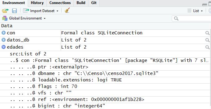
As you can see, even the row count is unavailable:
nrow(edades)## [1] NATo bring this column into RAM, use collect. I recommend always using it when you need a complete in-memory object rather than a database connection.
edades<-collect(edades)
nrow(edades)
## [1] 17574003edades## # A tibble: 17,574,003 x 1
## P09
## <int>
## 1 73
## 2 78
## 3 78
## 4 52
## 5 44
## 6 39
## 7 35
## 8 13
## 9 12
## 10 65
## # ... with 17,573,993 more rowsNow it works!
Another example: P09 represents age and P08 represents sex. Suppose we want the average age of men (sex = 1) by region. Do not forget collect!
hombres_edad <- datos_db %>%
  filter(P08==1) %>%
  group_by(REGION) %>%
  summarise(Edad_media = mean(P09))
hombres_edad <- collect(hombres_edad)
## Warning: Missing values are always removed in SQL.
## Use `AVG(x, na.rm = TRUE)` to silence this warninghombres_edad## # A tibble: 16 x 2
## REGION Edad_media
## <int> <dbl>
## 1 1 32.1
## 2 2 33.0
## 3 3 33.7
## 4 4 34.6
## 5 5 35.8
## 6 6 35.7
## 7 7 35.9
## 8 8 35.0
## 9 9 35.3
## 10 10 35.1
## 11 11 34.2
## 12 12 35.9
## 13 13 34.2
## 14 14 35.7
## 15 15 33.5
## 16 16 36.8We can now work with large structured datasets, retrieve subsets and perform analyses.
I hope you enjoyed this tutorial. Feel free to get in touch!


I am a data scientist and Natural Resources Engineer from Universidad de Chile, with a Master of Data Science from the University of Adelaide. I combine artificial intelligence, data science, statistical analysis and geospatial analysis to tackle environmental challenges.
Since February 2022, I have coordinated the Data Science team at Chile’s Superintendence of the Environment (SMA). I develop automation, data validation and analytical solutions for environmental monitoring and enforcement, using R, Python and SQL.
My experience also includes computer vision and deep learning for agricultural robotics, forest carbon modelling, remote sensing and survey data analysis. I have worked in Chile, Australia and Germany, combining applied research, algorithm development and interdisciplinary team coordination.